
Visualization Of 3D Data
The application program of choice is GNUplot. To demonstrate how to use gnuplot,
we will give an example.
The example will be to create a three dimensional plot of the Breit-Wigner
T-matrix:
where ER and Gamma are constants; ImE is the imaginary part
of the energy; Re E is the real part of the energy, and Im T is the imaginary
part of the T matrix. For this example, we will set ER = 180 MeV, Gamma = 120
MeV, Im E is the y axis, Re E is the x axis and Im T is the z axis.
Here is the C code I used to generate the data file in
the proper gnuplot format. The Data file consists of Z values calculated as a
function of x and y.
Here is the data file that I created with the above
code.
The most difficult area of gnuplot is producing a proper data file so GNUplot
can read it. We recommend producing a data file like this:
This file actually represents the coordinates of a matrix like this:
(This is a sample of a data file with only nine data points)
(x1 y1)
(x1 y2)
(x1 y3)
(x2 y1)
(x2 y2)
(x2 y3)
(x3 y1)
(x3 y2)
(x3 y3)
The blanklines represent the end of a row.
To make a data file to plot, copy and compile the above code or write your own.
To use the above code, you will need to redirect the standard output to a
file:
prompt> ./a.out > data
This will create a file called "data" in your current directory.
To start GNUplot, simply type:
prompt> gnuplot
To make a 3D surface plot of a file called "data" type:
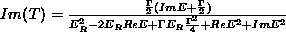
gnuplot> splot 'data'
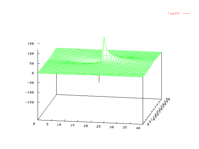
You should now have a plot which looks something like the plot below:
These plots usually don't look that good, it is better to use the lines
option.
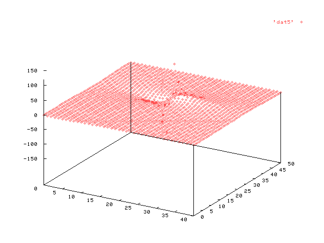
gnuplot> splot 'data' with lines
This will produce a plot like this:
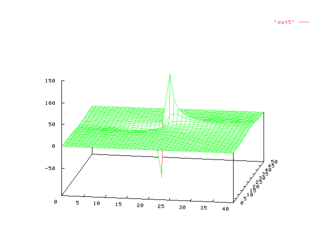
Plots like these still look a little confusing since you can't tell which part
is behind another. It is usually best to use the hidden 3d option.
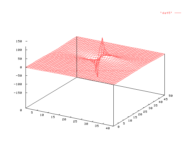
gnuplot> set hidden3d
gnuplot> splot 'data' with lines
The plot should now look like the plot below:
Now we can't see the bottom spike. To rotate the plot, we can use the set view
option:
gnuplot> set view 70,10
gnuplot> splot 'data' with lines
Now you will have a plot which looks like the plot below:
This sets the viewing angle to 70 degrees in the x direction and 10 degrees in
the z direction relative to the virtual coordinate system. For explanation of
this coordinate system, see the bottom of the tutorial.
Next, we can change the scaling on the z axis to elimanate the wasted space
below the plot:
gnuplot> set zrange [-25:150]
This option forces the specified axis to be in the specified range.
Here is the resultant plot:
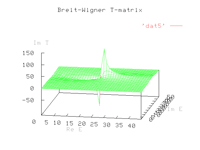
Now we are ready to label the axis and give the plot a title.
gnuplot>set xlabel "Re E"
gnuplot>set ylabel "Im E"
gnuplot>set zlabel "Im T"
gnuplot>set title "Breit-Wigner T-Matrix"
gnuplot>splot 'data' with lines
Here is the plot:
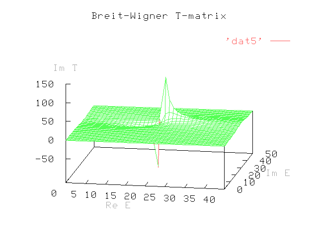
For this angle, the y axis tic marks seem too crowded so we would like to space
them 10 tics apart:
gnuplot> set ytics 0,10
gnuplot>splot 'data' with lines
Here is the plot:
Another option is to add contour lines to your plot. You can project them onto
the bottom of the plot and/or place them on the surface plot itself. The command
is:(NOTE: This plot will not yeild contours for some reason)
gnuplot> set contour base
or
gnuplot> set contour surface
or
gnuplot> set contour both
gnuplot> setgnuplot>help set view