References

1

The Undergraduate Computational Science And Engineering Project UCES, http://uces.ameslab.gov/.

2

The Northwest Alliance for Computational Science and Engineering NACSE, http://www.nero.net/nacse/.

3

Some samples can be seen at http://www webman@nacphy.physics.orst.edu/

4

Landau, R. H. and P. J. Fink, A Scientist's and Engineer's Guide to Workstations and Supercomputer, Wiley Interscience, New York, 1992.

5

http://www webman@nacphy.physics.orst.edu/ComPhys/MONTE/mc3/node6.html

  
Figure: Seven different randon walks. Each walk starts at the origin and makes 1000 steps. (Courtesy of P. Lagner.)

  
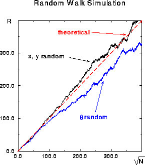
Figure: The distance R covered in random walks of N steps as a function of the square root of N. The solid curves correspond to two different techniques for simulating the random walks. (Courtesy of H. Kowallik.)

  
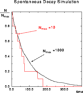
Figure: The fraction of nuclei remaining as a function of time in a simulation of radioactive decay. (Courtesy of H. Kowallik.)

  
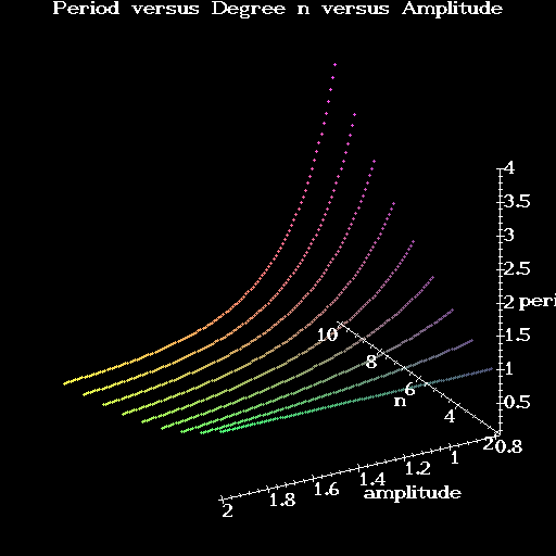
Figure: The period of an nth degree oscillator as a function of degree n and amplitude of oscillation. (Courtesy of P. Lagner.)