DATA ANALYSIS OF GPR AND APD DATA FROM ARCHAEOLOGICAL TELL SITES USING STATISTICAL DECONVOLUTION
Abstract
Creating accurate 3-D maps on complex archaeological sites is investigated. The process begins by applying (incoherent wave) pulses into the ground from the surface, digitizing the signals returning to the surface scattered from underground objects, and creating binary data files for each portion of the site. There is no utility in analysing these 'raw' data files directly, as the received signals are a tangle of the applied pulse shape and the scattering objects (that is, they are convolved). In order to re-create the scattering objects with their 3-D placement, a statistically-based deconvolution algorithm is employed. Although deconvolution algorithms are powerful, their statistical nature introduces parameters which do not have obvious meanings or predictable ranges of applicability. Once the 'raw' data has been deconvolved, processed data is saved as an hierarchical data format (HDF) file and disseminated.
Goal
Upon completion of this project, one should experience the challenges of using deconvolution algorithms with large data sets, including the affects of parameter choices. These algorithms utilize large matrices and matrix manipulations which are ripe for utilizing the power of parallel processing. A vital step in evaluating new algorithms and troubleshooting code is the use of simulated data, which is introduced. Another aspect to become comfortable with is the use of user-defined binary data files from actual experiments. User-defined data files are non-standard and often specific to the user's own software and programming style. We encourage in investigation of converting 'raw' files to standardized data files such as HDFs. Finally, the important dissemination of the processed data may be experienced by exploring 3-D viewing of the maps.
Background
To an archaeologist, a tell is series of buried structures such as governmental or military buildings, religious centers, or homes (1).
These buried structures are located at different depths depending on their date of use and are often overlapping either horizontally, vertically, or both. A cross-section of a tell is shown in Figure 1. Practicing archaeologists excavate tell sites to in an attempt to interpret the architecture, purpose, and date of occupation of the many structures contained within. This is, necessarily, a destructive investigation. In the interests of preservation, archaeologists have sought the help of physicists and geophysicists (2)
to develop non-destructive methods of mapping tell sites.
One popular method used by geophysicists to investigate sub-surface morphology is to define a survey grid for the site, position a pulsed wave source at the surface on the grid, and have one or more detectors located at other sites on the grid detect scattered signals. (3)
As the survey progresses, the locations of the source and detectors are alternated until the entire grid is covered. The result is a large series of data files containing the horizontal (x,y) coordinates along the grid and the signal strength versus time, or equivalently, the depth coordinate (z). Of course, different researchers collect the data and store it according to their own application rather than to any set standard.
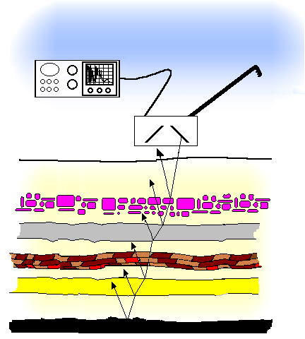
Figure 1
In these methods the (incoherent) wave source is typically pulsed such that many wavelengths of the mean frequency is contained within the pulse. Also, the 'length' of the pulse is often roughly the same as the distance between scatterers. Since there is a good likelihood that there are numerous layered scatterers underground, the received signals can be quite complicated. For instance, the reflection of five isolated scatterers of a typical ground-penetrating radar (GPR) pulse results in the received signal shown in Figure 2.
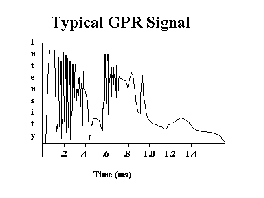
Figure 2
The Model
One model that can be used to give some comprehension to these complex signals is to employ linear systems theory (LST) (4).
LST does have its limitations when applied to a real physical system, but can provide a valuable starting point in the analysis of these signals. LST considers a 'system' to be a black box which 'operates' on input signals to creat output signals. See Figure 4. Mathematically, the inputs and outputs are descrtibed as functions and the system's response to inputs is understood to be an operator. The physicist knows many examples of operators applied to functions. For instance, recall the hydrogen atom's state function. Many of us are all too familiar with what happens when the Hamiltonian operator operates on this function! As far as LST is concerned, the outputs are the function produced when the applied inputs are operated on by the 'subversive' system.
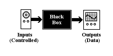
Figure 4
Imagine applying a single impulse to a system; an impulse lasting a differentially-short instant in time. We define the output one gets as the impulse response (or Green's) function for the system. Evidently, the impulse response function is related to the system operator. A system is linear if, for any arbitrary input, the output can be represented as a linear combination or superposition of the impulse response function and the inputs. Note that the superposition could indicate a sum or a superposition integral. This process of arriving at the output from a linear superposition of (products of) the input and impulse response function is called convolution.
Theory: Reflection Tomographic Analysis of Highly Directed, Pulsed Source Data
In geophysical techniques where highly directed pulsed source such as Ground Penetrating Radar (GPR) is used, a deconvolution scheme may be used to interpret data. The experiment involves applying a pulsed source which has a narrow and very slowing diverging beam. The source is situated on the ground surface, the pulse propagates downwards, scatters off the various discontinuities of the sub-surface, and returns to a detector which is (normally) situated at the same location of the pulsed source. An entire survey proceeds by moving the source and detector to alternate sites on a grid pattern on the ground surface. Data in the form of a 3-D matrix are produced; two dimensions describe the horizontal locations on the grid, one dimension describes the time dependent signal the detector receives. This is often the case with GPR experiments.
Placing some restrictions on the experiment can help to justify assumptions that will make it possible to employ simplistic models and analysis tools. The angular divergence of the beam (in radians) must not be larger than twice the wavelength divided by the depth of the deepest scatterer below the surface. This allows for the assumption that the detector will only receive signals from scatterers directly below it. At the least, it is hoped that the attenuation of the pulse is great enough that this criterion continues to be met until no detectable signal remains. It is also important that the typical vertical distance between scatterers be much longer than the 'carrier' frequency of the pulse envelope. If this criterion is not met, a diffraction model must be utilized instead of the much simpler reflection model for data analysis. In GPR, both these requirements are met. However, often the GPR pulse length is long compared with the vertical distance to the deepest scatterer. This is especially true in archaeological applications.
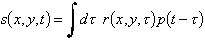
To set up both the theory and actual experiment, certain definitions must be made. Let there be a pulsed source signal which is applied to every location on a surface grid. The pulsed source, it is assumed, is consistent -- that is it is applied unvaryingly at each location on the grid. We call the pulse function as a function of time p(t). The grid will be defined with x-y axis corresponding to a know location on the ground. At regular intervals of Dx and Dy (and we set Dx = Dy as a matter of practice), we place the pulsed source at (x,y), or more correctly, ( i Dx, j Dy) where i,j are integers. The detector also placed at (x,y) detects a time-dependent signal s(x,y,t). In the actual experiment, this signal is digitized so that in reality the signal is discrete and has the form s( i Dx , j Dy, k Dt), where k is also an integer and Dt is the digitization period (or the reciprocal of sampling rate).
Evidently, the signal s(x,y,t) originated from the reflection of the pulse off a scattering layer. Let there be a function r = r(x,y,z) the represents then reflectivity of the sub-surface. It is expected that this function will be zero most of the time and strongly positive when there is a boundary between layers. An attenuating layer could also be indicated by slight negative values. Since all other functions have been discretised, the reflectivity would be r( form s( i Dx , j Dy, k c Dt), where c is the propagation velocity of the pulse.
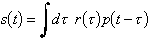
Since this a simple reflection model, it can be assumed that the signal received by the detector, s(x,y,t), is related to the pulse p(t) by the convolution of the pulse with the impulse response function of the sub-surface. Many researchers have made the claim that this convolution assumption is justified. Here, their lead is taken without discussion. Furthermore, it is recognized that the impulse response function is the reflectivity function defined above. Mathematically, then, the time-dependent received signal at location (x,y) on the grid is
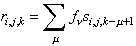
 Again, the actual (measured) functions are discrete. Using indices (i,j) to indicate the positions (x,y) and k to represent time (or distance via ct), the discrete convolution is written.
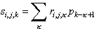 Here, i is in the range [1,Mi], j = [1,Mj], k = [1,Mk]. That is, the grid has Mi ´ Mj points and at each grid point Mk samples are taken at intervals of Dt.
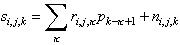
Closer to reality, there is added random noise ni,j,k so that
Here, i is in the range [1,Mi], j = [1,Mj], k = [1,Mk]. That is, the grid has Mi ´ Mj points and at each grid point Mk samples are taken at intervals of Dt.
Closer to reality, there is added random noise ni,j,k so that
 Now, how is the reflectivity function found? Recall that the received signals, s, are assumed to be the convolution between the reflection function, r, and the pulse function, p:
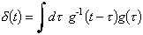
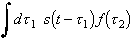
 Consider a 'filter function', f(t), which is somehow the inverse of the pulse function, p(t). Usually the inverse function would have the property that g-1g = 1. In this case, the "inverse function" has the following property:
 Contemplate this operation:
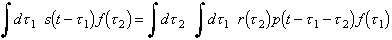
 Replacing s(t) with its representation as a convolution of p(t) and r(x,y,t):
 Let t' = t - t2
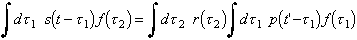 noting that due to the definition of f =p-1, the second integral is the delta function. This assumes that the integration has an upper limit of ¥ and lower limit of -¥ or at least that the integration covers all non-zero values of p(t) and f(t). In realistic situations, this is rarely difficult. Given the last step it is realized that the convolution of the received signals, s, and the filter, f, is simply the reflectivity function, r:
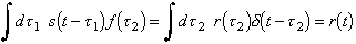 The last step above emphasises the fact that the reflectivity function is chosen to be the impulse response function or Green's function, that is, the response of the 'system' to a simple delta function input.
Of course, the actual functions are discrete, so the reflectivity may be expressed as
The last step above emphasises the fact that the reflectivity function is chosen to be the impulse response function or Green's function, that is, the response of the 'system' to a simple delta function input.
Of course, the actual functions are discrete, so the reflectivity may be expressed as
 with the total numbers of elements in the filter function is Mf. The length of the filter is arbitrary, but may have bearing on how well any deconvolution scheme functions.
A compelling reason for using this approach is that the reflectivity function may be found without knowledge of the pulse function. This is especially convenient as the pulse shape is not well know, if at all.
What if, by some serendipitous guess for a filter function, a very good estimate of the reflectivity function, restimated were found? A method of is needed to compare the actual function r with the estimated function, restimated; something like r - restimated is required. This has the smacking of an iterative approach: guess a filter function, compute the resulting reflectivity series, check the error, then try a new filter until the error becomes less than some preset small value. This is the approach taken by Wiggins (5-7) and Grey (8).
Borrowing from the field of statistics, the variance is a good predictor of the error. An example of this is computing the standard deviation of a set of averaged measurements. If the measurements fit a Gaussian distribution, the correct choice for the variance is the standard deviation.
The various discontinuities of the sub-surface which the pulse function interact with is assumed to be rather simple. As suggested earlier it is expected that there are only specular, (nearly) normal reflections at the boundaries between layers and no scattering, including diffractive scattering, from the material between these discontinuities. Luckily, with GPR experiments, this is typically true. Not discarding the possibility of attenuation via absorption, the expected reflection is 'spiky'. Figure 5, below shows a hypothetical series of layers and its reflectivity function.
with the total numbers of elements in the filter function is Mf. The length of the filter is arbitrary, but may have bearing on how well any deconvolution scheme functions.
A compelling reason for using this approach is that the reflectivity function may be found without knowledge of the pulse function. This is especially convenient as the pulse shape is not well know, if at all.
What if, by some serendipitous guess for a filter function, a very good estimate of the reflectivity function, restimated were found? A method of is needed to compare the actual function r with the estimated function, restimated; something like r - restimated is required. This has the smacking of an iterative approach: guess a filter function, compute the resulting reflectivity series, check the error, then try a new filter until the error becomes less than some preset small value. This is the approach taken by Wiggins (5-7) and Grey (8).
Borrowing from the field of statistics, the variance is a good predictor of the error. An example of this is computing the standard deviation of a set of averaged measurements. If the measurements fit a Gaussian distribution, the correct choice for the variance is the standard deviation.
The various discontinuities of the sub-surface which the pulse function interact with is assumed to be rather simple. As suggested earlier it is expected that there are only specular, (nearly) normal reflections at the boundaries between layers and no scattering, including diffractive scattering, from the material between these discontinuities. Luckily, with GPR experiments, this is typically true. Not discarding the possibility of attenuation via absorption, the expected reflection is 'spiky'. Figure 5, below shows a hypothetical series of layers and its reflectivity function.
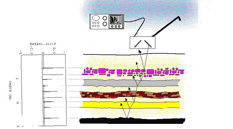
Figure 5
Note that attenuation due to the spreading out of beam is ignored. Ignoring the spreading out of the pulsed beam is justified, first since the beam divergence is intended to be small. Secondly, in the data collection equipment a time-dependent amplifier is employed typically with an exponentially increasing gain. Perhaps it should be pointed that usually researchers are less interested in the strength of the reflectivity than they are in the three-dimensional location of reflecting boundaries and their orientation with respect to each other. Should an exact value for the reflectivity be needed, more a priori information is required such as the amplifier gain, detector response, typical dispersion and frequency-dependent absorption of the media in the layers, and possibly other experimental parameters.
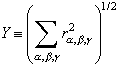
The approach taken by some researches (5-14) is to compute an approximation to the reflections function by minimizing a variance associated with 'spiky' data. Since the aim is to arrive at a reflection function that has a simple, spiky distribution, this approach is referred to as minimum entropy deconvolution. There are several suggestions to variances of spiky distributions in the literature including Wiggin's Varimax norm (or V norm) and Grey's Wiggins-Type norm (or G norm). Cabrelli (12) suggested a variance associated with 'spiky' distribution is the D norm:
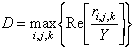
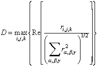 where the max function steps through all the indices i,j,k and returns the maximum element in the matrix in the square brackets. In an iterative computation, a new filter is proposed based on the failure or success of the previous iteration, the reflection function is computed, and the reflectivity distribution's variance is tabulated. As the iterative computation proceeds the variance changes as suggested in Figure 6. The process is terminated when the minimum variance or 'entropy' is achieved.
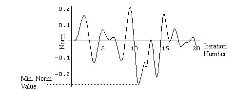 Figure 6
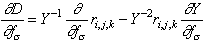
Cabrelli had the insight that the minimum of the variance (his D norm) could be found by the usual method in calculus: set the derivative of the function, that is the variance, with respect to the filter function to zero and solve the equation for the reflectivity function.
First, let
Figure 6
Cabrelli had the insight that the minimum of the variance (his D norm) could be found by the usual method in calculus: set the derivative of the function, that is the variance, with respect to the filter function to zero and solve the equation for the reflectivity function.
First, let
 so that the norm is
 then the derivative of D with respect to element /sigma in the filter vector is
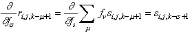
 The individual derivatives are
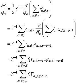 where it is recognized that the expression
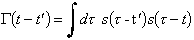
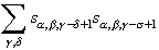 is the autocorrelation function G. Usually it written in integral form:
 Finally, the derivative of the D norm is
 Now, setting the derivative to zero, it is seen that
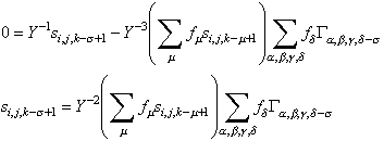 This is a rather exasperating expression until it is recast by recognizing that if
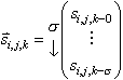
 where d-s is in the range [-Mf, Mf] (elements of R for d-s not in that range are defined as zero) and if
 Then, the equation that produces a reflectivity function which is simple and spiky becomes
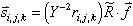 Now the above vector equation can be solved for the filter function creating a non-iterative way to compute the filter:
 If the above is a valid solution, it can be argued that another perfectly good solution should be
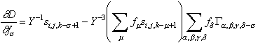
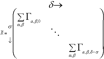
 Once the filter is computed, from the matrix of autocorrelations of the received signals, R, and the vector of received signals, it can be used to calculate the reflectivity function. This expression is ripe for numerical computation with the right vector and matrix handling routines. In fact, looking at the definition for R it is has the triangle-like symmetry of a Toeplitz matrix which can be inverted using a Levinson recursion algorithm.
Results
References
1 The Practical Archaeologist
2 Archaeological Applications of Remote Sensing, Conference, Boston
3 Waters, Reflection Siesmology, Wiley
4 Gaskill, Linear Systems, Fourier Tranforms, and Optics, Wiley
5 R. A. Wiggins, Minimum entropy deconvolution, Geoexpl., 16, pp. 21-35, 1978.
6 A. Jurkevics, R. Wiggins, A critique of seismic deconvolution methods, Geophys. 49, pp. 2109-2116, 1984.
7 R. A. Wiggins, Entropy guided deconvolution, Geophys., 50, pp. 2720-2726, 1985.
8 W. C. Gray, Variable norm deconvolution: Ph.D, thesis, Stanford Univ.
9 T. J. Ulrych, C. Walker, Analytical minimum entropy deconvolution, 47, pp.1295-1302, 1982.
10 M. Ooe, T. J. Ulrych, Minimum entropy deconvolution with an exponential transformation, Geophys., 27, pp. 458-473, 1979.
11 J. S. C. Fung, A. N. Venetsanopoulos, Design of quadratic filters based on the D norm for seismic deconvolution, IEEE signal processing conference proceedings, 1987.
12 C. A. Cabrelli, Minimum entropy deconvolution and simplicity: A noniterative algorithm, Geophys., 50, pp. 394-413, 1984.
13 A. T. Walden, A comparison of stochastic gradient and minimum entropy deconvolution algorithms, Signal Processing, 15, pp. 203-211, 1988.
14 T. J. Ulrych, C. J. Walker, A. J. Jurkevics, A filter length criterion for minimum entropy deconvolution, J. of Canadian Soc. of Exploration Geophysics, 14, pp. 21-28, 1978.