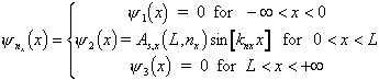
We consider a 3-D box of dimensions L. Inside the box the potential is zero. Outside the box the potential is infinity. Use the results of the example, The 1-D Infinite Square Well With A Non-Zero Bottom and the lab An Infinite Square Well With A Non-Zero Bottoms.

1. Read in a set of useful functions by executing a cell containing:

(You may need to FTP or move this useful.ma file to the Mathematica main directory first.)

1. Define the Hermitian Conjugate (HC) of a complex function using the built-in Conjugate function as

1. Some constants are only real numbers. To force Mathematica to treat the following important constants, variables, functions, and quantum numbers execute the following cell:

Clear[L];

RealOnly[L];

RealOnly[x];

RealOnly[y];

RealOnly[z];

RealOnly[nx];

RealOnly[ny];

RealOnly[nz];

1. Create a function that will compute the expectation value (y*y) of x for an eigenfunction y (as yet undefined) with variables x, y, z, nx, ny, and nz. (Don't define psi or L yet.) Example:

Clear[xmean];

RealOnly[xmean];

xmean[nx_,ny_,nz_,As_] : = Simplify[1/As^2 Integrate[

HC[psi[x,y,z,nx,ny,nz]] x psi[x,y,z,nx,ny,nz],{x,0,L},{y,0,L},{z,0,L}]]

Note that the "x" in the above line is 'not times' its 'multiply by x'. Why are we insisting that the expectation value of x be only real?

1. Don't do it, just answer the questions:
   1. How would you create a function that computes the expectation value of ?
   2. For ?
2. Create a function that will compute the expectation values of x² using step 4 as a template.

Save your work!

1. Create functions that will compute the expectation values and . Please don't define hbar, just leave it as hbar. Hint: To compute the n^th partial derivative of f(x,y) with respect to x, do this:

1. The state (or wave) function for a particle in a 1-D box along the x axis with quantum number n_x is

Please note: n_x = (1,2,...); n_x = 0 is not state.

Analytically, on a slip of paper (preferably the back of an envelope), agree upon the state function for a 3-D box centered about x = L/2, y = L/2, and z = L/2. Remember the 'separation of dimensions in DEs' discussion we participated in.

Save your work!

1. Without worrying about normalization (will put that into another function), define the particle's wave function of energy eigenstate, y, for all three dimensions. I want you to call psi in a certain way as the hint below suggests:

1. Compute the inverse square of the constant of normalization "A_s":

norm = Simplify[Integrate[

HC[psi[x,y,z, 1,1,1]] psi[x,y, z, 1, 1, 1]

,{x,0,L},{y,0,L},{z,0,L}]]

Note that it is done explicitly for the state nx = 1, ny = 1, nz = 1. This is for computational speed. If you left the state as a general (without specifying the n's) Mathematica would eventually compute it, but why wait? (If this doesn't not give the right results, then define a function for As, which will have input parameters of L and nx, ny, nz. )

Save your work!

1. Define a function that computes the probability of finding the particle with a state (nx, ny, nz) in the box at location (x,y,z). Call it psi2; below is a hint of what it might look like:

Clear[psi2]

RealOnly[psi2];

As = 1/norm;

psi2[x_,y_,z_,nx_,ny_,nz_, norm_] : = As ...

Note that I put the variable norm = 1/(As) as computed in a previous step.

Save your work!

1. Test to be sure the normalization is correct. Check it for state (nx=2, ny = 1, nz = 1) for kicks:

Simplify[Integrate[ psi2[x,y,z,2,1,1,As],{x,0,L},{y,0,L},{z,0,L}]]

Also try it for one to two other states to be certain that our normalization factor As isn't state-dependent.

DO THIS SECTION ONLY IF TIME ALLOWS ------------------------------------------------------------

1. For the lowest possible energy state, find , , and .

1. Find , , and for the lowest possible energy state.

Save your work!

1. Compute . Is it consistent with Heisenberg's Uncertainty Principle?

Save your work!

1. Copy the cells containing your work for steps 13-0. Edit the copy and repeat the steps for the energy state nx = 2, ny = 1, nz = 1. Repeat these calculations for these edited steps.

END OF DO THIS SECTION ONLY IF TIME ALLOWS ---------------------------------------------------------

1. Create a function that will compute the energy eigenvalue for a state psi and any quantum numbers nx, ny, nz. For this you must figure out how to write the Hamiltonian and the appropriate matrix element. Recall H = -p²/(2m). Here the p is the operator p. Don't define m.
2. Compute the energies for , , , and . Clearly these are different states (use can explore them by plotting -- later). Question: What fold-degenerate are each of these energy eigenvalues?

Save your work!

1. Plot the probability of finding the particle at an x-position from 0 to L (and both y and z at L/2), with L = 10 for states (1,1,1), (2,1,1), and (3,1,1). Your cell should look as shown below. Be sure to reset L when you are done.

L = 10;

Plot[ { psi2[x,L/2,L/2,1,1,1,As],

psi2[x,L/2,L/2,2,1,1,As],

psi2[x,L/2,L/2,3,1,1,As]},{x,0,L}]

Clear[L];

RealOnly[L];

1. For fun, use

L = 10;

PL1 = Plot3D[ psi2[x,y,L/2, 2,1,1,As], {x,0,L},{y,0,L}]

Clear[L];

RealOnly[L];

to plot the probability of finding the particle at an x and y position from 0 to L (and z at L/2), with L = 10 for state(2,1,1). Note that the plot's directives are saved in variable "PL1".

Save your work!

1. The function

Show[PL1,ViewPoint->{5.657,0.000,1.250}]

will redraw the plot (saved as "PL1") in step 20 at a different orientation. Try it.

1. For a real thrill, let's make an animation of (the second) step 20. We can show the probability surface plot from different angles as done above. The best way to see the entire surface is to rotate the plot 360 degrees about the z-axis. First we redraw the view in several different orientations, then we highlight the cells with the views and press the 'animate' button on the toolbar. Its looks like a frame from a movie reel. I'll save you the time of typing out all the views. Open the file: "PH312LABd.ma" and copy the cell to your notebook. It might also be available from the web site and you can cut and paste it over to your notebook. It should look like this:

Show[PL1,ViewPoint->{5.657,0.000,1.250}]

Show[PL1,ViewPoint->{5.137,2.368,1.250}]

Show[PL1,ViewPoint->{2.686,4.978,1.250}]

Show[PL1,ViewPoint->{0.133,5.655,1.250}]

Show[PL1,ViewPoint->{-2.528,5.060,1.250}]

Show[PL1,ViewPoint->{-5.209,2.206,1.250}]

Show[PL1,ViewPoint->{-5.337,-1.874,1.250}]

Show[PL1,ViewPoint->{-4.273,-3.708,1.250}]

Show[PL1,ViewPoint->{-2.608,-5.020,1.250}]

Show[PL1,ViewPoint->{-0.222,-5.652,1.250}]

Show[PL1,ViewPoint->{2.206,-5.209,1.250}]

Show[PL1,ViewPoint->{4.214,-3.774,1.250}]

To save space, you might want to remove the cell you executed in step 0. Before proceeding, save your notebook! Execute the cell above. When its complete, you should have a dozen plots. Highlight all the cells (from the blue cell bar at the right) containing these plots. Press the animate button! It was worth the effort. If you think this is cool, just wait!

1. This is a book keeping step. Save your notebook. Then save it under another file name. Since the plots take up so much space, delete all the plots and re-save this new notebook. Then make a second copy this file called later.ma. You will use the file, um, later this term. Finally, re-open the first file and proceed to the next step.

The next several steps are an attempt to create a scatter plot of the probability versus 3D space. The plot will indicate high probability of the particle's location with a high density of dots and a low probability with a low density of dots. We will use this code again, slightly modified, in studying the electron probability clouds for a hydrogen atom. The plot requires a module called 'SctrPlot.ma' and some preparation.

1. We are about to do some numerical computations. Set hbar = 1, L = 10, and m = 1. This is a particular set of units called 'natural units'. By the way, c = 1 in these units also. Now force psi to be numerical by copying the old function for psi, then putting it inside the 'make it numerical', N[ ] function. The new version of the cell containing psi should look like this:

Clear[ psi]

psi2[x_,y_, z_, nx_, ny_, nz_]:=

N[ ...your old code for psi goes here... ]

Before you continue, call me over and show me that a cell like the one below returns a numerical value:

psi2[ .3 L, .3 L, .3 L, 1, 1, 1]

Save your work!

1. Read in the SctrPlot module by executing a cell containing

<<Sctrplot.ma

From the documentation for SctrPlot:

ScatterPlot -- a module which takes a function psi2[x,y,x,nx,ny,nz,A] and creates an array of points with the highest density of points where psi2 is large in a space [x,y,z]. psi2 is suppose to represent a wavefunction^.

Syntax: ScatterPlot[nx, ny, nz, MinL, MaxL, maxintervals, maxloops, maxinlastrange]

nx,ny,nz are for the quantum numbers

minL and maxL are the expected boundaries of the plot. L could is the effective dimensions of the box, or just the min and max values for the plot.

maxintervals is used only for finding the maximum value of the psi2 function. Choose it to be the smallest you can, but it the derivative is big it stops, you may need to make larger. Suggested range: 100 to 1000.

maxloops = the max number of loops try 5K for fast & dirty, but you may need more depending on your setting for

maxinlastrange which the factor that determines the accuracy. If maxloops is too small, you may get a message the maxinlastrange to too small. Essentially this parameter puts this number of points where they have a probability from 0.9 to 1.0. Speed is slow id you have a large number for this parameter, but if it is too small, much detail in the picture will be lost.

1. Now, it will take some time to execute a cell like that shown below. The command will plot the probability in 3D for state (1,1,1). The execution time varies, but you might as well go get a cup of coffee or take a walk rather than wait around.

stcplt = ScatterPlot[1,1,1,0,L,2,10000,100];

Once you have been able to successfully execute the above cell, try for a more accurate computation by editing the cell so it looks like this:

stcplt = ScatterPlot[1,1,1,0,L,2,10000,1000];

Save your work!

1. Without executing the cells, type in the commands to show the scatter plot for states (2,1,1) and (2,2,1). Perhaps you can divide these plots among other in the class. You should also try two more states, although I wouldn't try higher states than (4,4,4). When you are done editing. Save your work (again). Save the work on a disk. Highlight all the new cells and execute them. If they don't complete by the end of class, I'll take them to my server and execute them for a day and see the results later. HINT: You'll need to change stcplt = ScatterPlot[1,1,1,0,L,2,10000,1000]; so that the "2" after the "L" is larger. I'd suggest that you choose this parameter to be 2 times the largest value of nx, ny, or nz.

I haven't tried increasing maxinlastrange larger than 1000. Maybe you should try 5000 and increase maxloops accordingly.

Finally, we should look at all the plots and try to understand what they are tell us. Be certain you write a paragraph concerning our discussion in you report.